Advanced Data Manipulation with R
Data analysis involves a large amount of janitor work - munging and cleaning data to facilitate downstream data analysis. This workshop assumes you have a basic familiarity with R and want to learn tools and techniques for advanced data manipulation. It will cover data cleaning and "tidy data," and will introduce R packages that enable data manipulation, analysis, and visualization using split-apply-combine strategies. Upon completing this lesson, you will be able to use the dplyr package in R to effectively manipulate and conditionally compute summary statistics over subsets of a "big" dataset containing many observations.
This is not a beginner course. This workshop requires basic familiarity with R: data types including vectors and data frames, importing/exporting data, and plotting. You can refresh your R knowledge with DataCamp's Intro to R or TryR from CodeSchool.
Before coming
You'll need to bring a laptop to the course with the software installed as detailed below.
Note: R and RStudio are separate downloads and installations. R is the underlying statistical computing environment, but using R alone is no fun. RStudio is a graphical integrated development environment that makes using R much easier. You need R installed before you install RStudio.
- Download data. Download the
gapminder.csvandmalebmi.csvfiles from bioconnector.org/data. Save them somewhere easy to find. Optionally, open them up in Excel and look around. - Install R. You'll need R version 3.1.2 or higher. Download and install R for Windows or Mac OS X (download the latest R-3.x.x.pkg file for your appropriate version of OS X).
- Install RStudio. Download and install the latest stable version of RStudio Desktop. Alternatively, download the RStudio Desktop v0.99 preview release (the 0.99 preview version has many nice new features that are especially useful for this particular workshop).
- Install R packages. Launch RStudio (RStudio, not R itself). Ensure that you have internet access, then enter the following commands into the Console panel (usually the lower-left panel, by default). Note that these commands are case-sensitive. At any point (especially if you've used R/Bioconductor in the past), R may ask you if you want to update any old packages by asking
Update all/some/none? [a/s/n]:. If you see this, typeaat the propt and hitEnterto update any old packages. If you're using a Windows machine you might get some errors about not having permission to modify the existing libraries -- don't worry about this message. You can avoid this error altogether by running RStudio as an administrator.
# Install packages from CRAN
install.packages("dplyr")
install.packages("ggplot2")
install.packages("tidyr")
install.packages("knitr")
install.packages("rmarkdown")
You can check that you've installed everything correctly by closing and reopening RStudio and entering the following commands at the console window:
library(dplyr)
library(ggplot2)
library(tidyr)
library(knitr)
library(rmarkdown)
These commands may produce some notes or other output, but as long as they work without an error message, you're good to go. If you get a message that says something like: Error in library(packageName) : there is no package called 'packageName', then the required packages did not install correctly. Please do not hesitate to email me prior to the course if you are still having difficulty.
Review
We use data frames to store heterogeneous tabular data in R: tabular, meaning that individuals or observations are typically represented in rows, while variables or features are represented as columns; heterogeneous, meaning that columns/features/variables can be different classes (on variable, e.g. age, can be numeric, while another, e.g., cause of death, can be text).
Before coming, you should have downloaded the gapminder data. If you downloaded this entire lesson repository, once you extract it you'll find it in workshops/lessons/r/data/gapminder.csv. Alternatively you can download it directly from http://bioconnector.org/data/. This dataset is an excerpt from the Gapminder data, that's already been cleaned up to a degree. This particular dataset has 1704 observations on six variables:
countrya categorical variable (aka "factor") 142 levelscontinent, a categorical variable with 5 levelsyear: going from 1952 to 2007 in increments of 5 yearspop: populationgdpPercap: GDP per capitalifeExp: life expectancy
Let's load the data first. There are two ways to do this. You can use RStudio's menus to select a file from your computer (tools, import dataset, from text file). But that's not reproducible. The best way to do this is to save the data and the script you're using to the same place, and read in the data in using read.csv. It's important to tell R that the file has a header, which tells R the names of the columns. We tell this to R with the header=TRUE argument.
Once we've loaded it we can type the name of the object itself (gm) to view the entire data frame. Note: doing this with large data frames can cause you trouble.
gm <- read.csv("data/gapminder.csv", header=TRUE)

# Alternatively, read directly from the web:
# gm <- read.csv(url("http://bioconnector.org/data/gapminder.csv"), header=TRUE)

class(gm)
gm
There are several built-in functions that are useful for working with data frames.
- Content:
head(): shows the first 6 rowstail(): shows the last 6 rows
- Size:
dim(): returns a 2-element vector with the number of rows in the first element, and the number of columns as the second element (the dimensions of the object)nrow(): returns the number of rowsncol(): returns the number of columns
- Summary:
colnames()(or justnames()): returns the column namesstr(): structure of the object and information about the class, length and content of each columnsummary(): works differently depending on what kind of object you pass to it. Passing a data frame to thesummary()function prints out some summary statistics about each column (min, max, median, mean, etc.)
head(gm)
tail(gm)
dim(gm)
nrow(gm)
ncol(gm)
colnames(gm)
str(gm)
summary(gm)
View(gm)
The dplyr package
The dplyr package is a relatively new R package that makes data manipulation fast and easy. It imports functionality from another package called magrittr that allows you to chain commands together into a pipeline that will completely change the way you write R code such that you're writing code the way you're thinking about the problem.
tbl_df
Let's go back to our gapminder data. It's currently stored in an object called gm. Remember that gm is a data.frame object if we look at its class(). Also, remember what happens if we try to display gm on the screen? It's too big to show us and it fills up our console.
class(gm)
gm
The first really nice thing about the dplyr package is the tbl_df class. A tbl_df is basically an improved version of the data.frame object. The main advantage to using a tbl_df over a regular data frame is the printing: tbl objects only print a few rows and all the columns that fit on one screen, describing the rest of it as text. We can turn our gm data frame into a tbl_df using the tbl_df() function. Let's do that, and reassign the result back to gm. Now, if we take a look at gm's class, we'll see that it's still a data frame, but it's also now a tbl_df. If we now type the name of the object, it will by default only print out a few lines. If this was a "wide" dataset with many columns, it would also not try to show us everything.
library(dplyr)
gm <- tbl_df(gm)
class(gm)
gm
You don't have to turn all your data.frame objects into tbl_df objects, but it does make working with large datasets a bit easier.
EXERCISE 1
Load the malebmi.csv data. This is male BMI data from 1980 through 2008 from the gapminder project. If you downloaded the zip file from the repository, it's located in workshops/lessons/r/data. Alternatively you can donload it directly from http://bioconnector.org/data/.
- Load this into a data frame object called
bmi. - Turn it into a
tbl_df. - How many rows and columns does it have?
Don't remove it -- we're going to use it later on.
dplyr verbs
The dplyr package gives you a handful of useful verbs for managing data. On their own they don't do anything that base R can't do.
- filter
- select
- mutate
- arrange
- summarize
- group_by
- more later...
They all take a data.frame or tbl_df as their input for the first argument.
filter()
First, this is from the introduction lecture, if you want to filter rows of the data where some condition is true, use the filter() function. The first argument is the data frame or tbl, and the second argument is the condition you want to satisfy.
# Show only stats for the year 1982
filter(gm, year==1982)

# Show only stats for the US
filter(gm, country=="United States")

# Show only stats for American contries in 1997
filter(gm, continent=="Americas" & year==1997)

# Show only stats for countries with per-capita GDP of less than 300 OR a
# life expectancy of less than 30. What happened those years?
filter(gm, gdpPercap<300 | lifeExp<30)
select()
The filter() function allows you to return only certain rows matching a condition. The select() function lets you subset the data and restrict to a number of columns. The first argument is the data, and subsequent arguments are the columns you want. Let's just get the year and the population variables.
select(gm, year, pop)
mutate()
The mutate() function adds new columns to the data. Remember, the variable in our dataset is GDP per capita, which is the total GDP divided by the population size for that country, for that year. Let's mutate this dataset and add a column called gdp:
mutate(gm, gdp=pop*gdpPercap)
Mutate has a nice little feature too in that it's "lazy." You can mutate and add one variable, then continue mutating to add more variables based on that variable. Let's make another column that's GDP in billions.
mutate(gm, gdp=pop*gdpPercap, gdpBil=gdp/1e9)
arrange()
The arrange() function does what it sounds like. It takes a data frame or tbl and arranges (or sorts) by column(s) of interest. The first argument is the data, and subsequent arguments are columns to sort on. Use the desc() function to arrange by descending.
arrange(gm, lifeExp)
arrange(gm, year, desc(lifeExp))
summarize()
The summarize() function summarizes multiple values to a single value. On its own the summarize() function doesn't seem to be all that useful.
summarize(gm, mean(pop))
summarize(gm, meanpop=mean(pop))
summarize(gm, n())
summarize(gm, n_distinct(country))
group_by()
We saw that summarize() isn't that useful on its own. Neither is group_by() All this does is takes an existing tbl and coverts it into a grouped tbl where operations are performed by group.
gm
group_by(gm, continent)
class(group_by(gm, continent))
The real power comes in where group_by() and summarize() are used together. Let's take the same grouped tbl from last time, and pass all that as an input to summarize, where we get the mean population size. We can also group by more than one variable.
summarize(group_by(gm, continent), mean(pop))

group_by(gm, continent, year)
summarize(group_by(gm, continent, year), mean(pop))
The almighty pipe: %>%
This is where things get awesome. The dplyr package imports functionality from the magrittr package that lets you pipe the output of one function to the input of another, so you can avoid nesting functions. It looks like this: %>%. You don't have to load the magrittr package to use it since dplyr imports its functionality when you load the dplyr package.
Here's the simplest way to use it. Think of the head() function. It expects a data frame as input, and the next argument is the number of lines to print. These two commands are identical:
head(gm, 5)
## Source: local data frame [5 x 6]
##
##       country continent year lifeExp      pop gdpPercap
## 1 Afghanistan      Asia 1952    28.8  8425333       779
## 2 Afghanistan      Asia 1957    30.3  9240934       821
## 3 Afghanistan      Asia 1962    32.0 10267083       853
## 4 Afghanistan      Asia 1967    34.0 11537966       836
## 5 Afghanistan      Asia 1972    36.1 13079460       740
gm %>% head(5)
## Source: local data frame [5 x 6]
##
##       country continent year lifeExp      pop gdpPercap
## 1 Afghanistan      Asia 1952    28.8  8425333       779
## 2 Afghanistan      Asia 1957    30.3  9240934       821
## 3 Afghanistan      Asia 1962    32.0 10267083       853
## 4 Afghanistan      Asia 1967    34.0 11537966       836
## 5 Afghanistan      Asia 1972    36.1 13079460       740
So what?
Now, think about this for a minute. What if we wanted to get the life expectancy and GDP averaged across all Asian countries for each year? (See top of image). Mentally we would do something like this:
- Take the
gmdataset mutate()it to add raw GDPfilter()it to restrict to Asian countries onlygroup_by()year- and
summarize()it to get the mean life expectancy and mean GDP.
But in code, it gets ugly. First, mutate the data to add GDP.
mutate(gm, gdp=gdpPercap*pop)
Wrap that whole command with filter().
filter(mutate(gm, gdp=gdpPercap*pop), continent=="Asia")
Wrap that again with group_by():
group_by(filter(mutate(gm, gdp=gdpPercap*pop), continent=="Asia"), year)
Finally, wrap everything with summarize():
summarize(
  group_by(
    filter(
      mutate(gm, gdp=gdpPercap*pop),
    continent=="Asia"),
  year),
mean(lifeExp), mean(gdp))
Now compare that with the mental process of what you're actually trying to accomplish. The way you would do this without pipes is completely inside-out and backwards from the way you express in words and in thought what you want to do. The pipe operator %>% allows you to pass data frame or tbl objects from one function to another, so long as those functions expect data frames or tables as input.
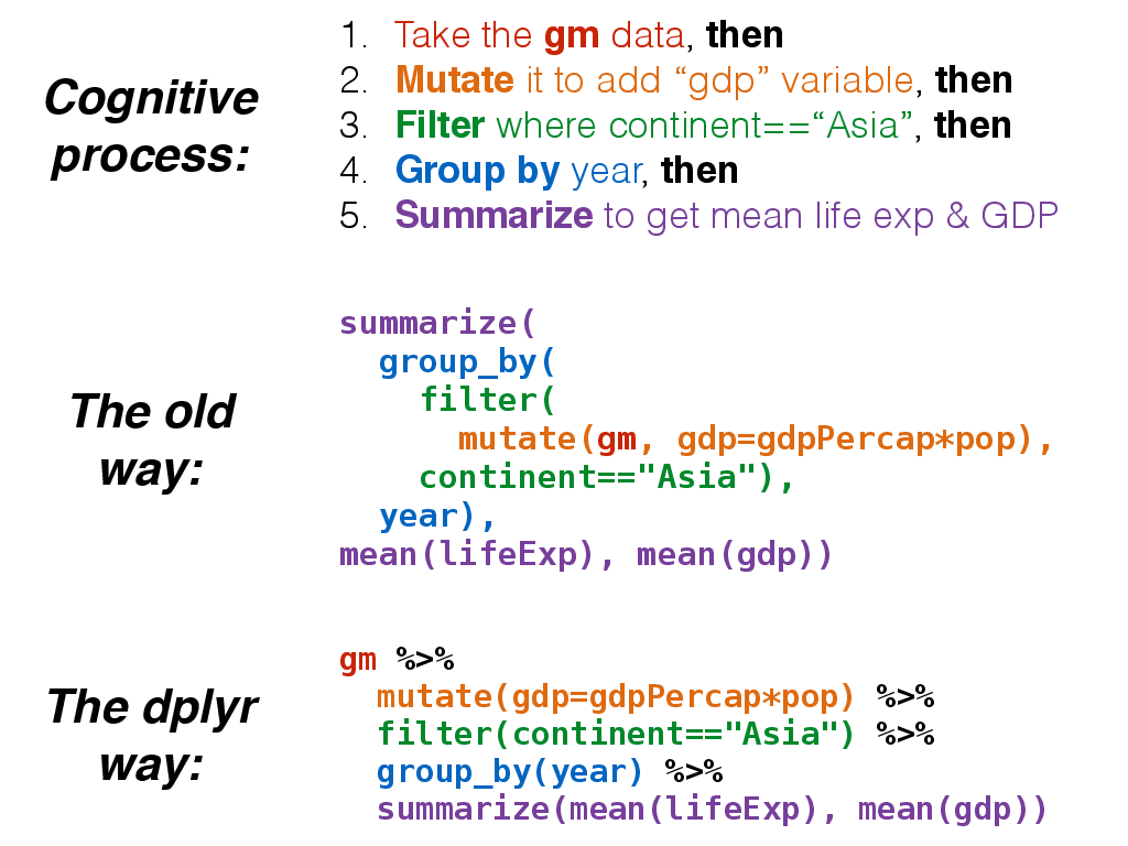
This is how we would do that in code. It's as simple as replacing the word "then" in words to the symbol %>% in code.
gm %>%
  mutate(gdp=gdpPercap*pop) %>%
  filter(continent=="Asia") %>%
  group_by(year) %>%
  summarize(mean(lifeExp), mean(gdp))
EXERCISE 2
Here's a warm-up round. Try the following.
What was the population of Peru in 1992? Show only the population variable. Hint: 2 pipes; use filter and select.
## Source: local data frame [1 x 1]
##
##        pop
## 1 22430449
Which countries and which years had the worst five GDP per capita measurements? Hint: 2 pipes; use arrange and head.
## Source: local data frame [5 x 6]
##
##            country continent year lifeExp      pop gdpPercap
## 1 Congo, Dem. Rep.    Africa 2002    45.0 55379852       241
## 2 Congo, Dem. Rep.    Africa 2007    46.5 64606759       278
## 3          Lesotho    Africa 1952    42.1   748747       299
## 4    Guinea-Bissau    Africa 1952    32.5   580653       300
## 5 Congo, Dem. Rep.    Africa 1997    42.6 47798986       312
What was the average life expectancy across all contries for each year in the dataset? Hint: 2 pipes; group by and summarize.
## Source: local data frame [12 x 2]
##
##    year mean(lifeExp)
## 1  1952          49.1
## 2  1957          51.5
## 3  1962          53.6
## 4  1967          55.7
## 5  1972          57.6
## 6  1977          59.6
## 7  1982          61.5
## 8  1987          63.2
## 9  1992          64.2
## 10 1997          65.0
## 11 2002          65.7
## 12 2007          67.0
That was easy, right? How about some tougher ones.
EXERCISE 3
Which five Asian countries had the highest life expectancy in 2007? Hint: 3 pipes.
## Source: local data frame [5 x 6]
##
##            country continent year lifeExp       pop gdpPercap
## 1            Japan      Asia 2007    82.6 127467972     31656
## 2 Hong Kong, China      Asia 2007    82.2   6980412     39725
## 3           Israel      Asia 2007    80.7   6426679     25523
## 4        Singapore      Asia 2007    80.0   4553009     47143
## 5      Korea, Rep.      Asia 2007    78.6  49044790     23348
How many countries are on each continent? Hint: 2 pipes.
## Source: local data frame [5 x 2]
##
##   continent n_distinct(country)
## 1    Africa                  52
## 2  Americas                  25
## 3      Asia                  33
## 4    Europe                  30
## 5   Oceania                   2
Separately for each year, compute the correlation coefficients (e.g., cor(x,y)) for life expectancy (y) against both log10 of the population size and log10 of the per capita GDP. What do these trends mean? Hint: 2 pipes.
## Source: local data frame [12 x 3]
##
##    year cor(log10(pop), lifeExp) cor(log10(gdpPercap), lifeExp)
## 1  1952                   0.1543                          0.748
## 2  1957                   0.1584                          0.759
## 3  1962                   0.1376                          0.771
## 4  1967                   0.1482                          0.773
## 5  1972                   0.1322                          0.789
## 6  1977                   0.1142                          0.814
## 7  1982                   0.0944                          0.846
## 8  1987                   0.0732                          0.874
## 9  1992                   0.0593                          0.856
## 10 1997                   0.0636                          0.864
## 11 2002                   0.0746                          0.825
## 12 2007                   0.0653                          0.809
Compute the average GDP (not per-capita) in billions averaged across all contries separately for each continent separately for each year. What continents/years had the top 5 overall GDP? Hint: 6 pipes. If you want to arrange a dataset by a value computed on grouped data, you first have to pass that resulting dataset to a funcion called ungroup() before continuing to operate.
## Source: local data frame [5 x 3]
##
##   continent year meangdp
## 1  Americas 2007     777
## 2  Americas 2002     661
## 3      Asia 2007     628
## 4  Americas 1997     583
## 5    Europe 2007     493
Tidy data
So far we've dealt exclusively with tidy data - data that's easy to work with, manipulate, and visualize. That's because our gapminder dataset has two key properties:
- Each column is a variable.
- Each row is an observation.
You can read a lot more about tidy data in this paper. Let's load some untidy data and see if we can see the difference. This is some made-up data for five different patients (Jon, Ann, Bill, Kate, and Joe) given three different drugs (A, B, and C), and measuring their heart rate. If you didn't download the entire lesson repository from GitHub, you can download the heartrate.csv file directly from http://bioconnector.org/data/.
hr <- read.csv("data/heartrate.csv")
hr
Notice how with the gapminder data each variable, country, continent, year, lifeExp, pop, and gdpPercap, were each in their own column. In the heart rate data, we have three variables: name, drug, and heart rate. Name is in a column, But drug is in the top row, and heart rate is scattered around the entire table. If we wanted to do things like filter the dataset where drug=="a" or heartrate>=80 we couldn't do it because these variables aren't in columns.
The tidyr package helps with this. There are other functions in the tidyr package but one particularly handy one is the gather() function, which takes multiple columns, and gathers them into key-value pairs: it makes "wide" data longer. We can get a little help with ?gather.
library(tidyr)
hr %>% gather(key=drug, value=heartreate, a,b,c)
hr %>% gather(key=drug, value=heartreate, -name)
If we create a new data frame that's a tidy version of hr, we can do those kinds of manipulations we talked about before
# Create a new data.frame
hrtidy <- hr %>%
  gather(key=drug, value=heartrate, -name)
hrtidy

# filter
hrtidy %>% filter(drug=="a")
hrtidy %>% filter(heartrate>=80)

# analyze
hrtidy %>%
  group_by(drug) %>%
  summarize(mean(heartrate))
Two-table verbs
It's rare that a data analysis involves only a single table of data. You normally have many tables that contribute to an analysis, and you need flexible tools to combine them. The dplyr package has several tools that let you work with multiple tables at once. The most straightforward one is the inner_join.
First, let's read in some BMI data from the gapminder project. This is the average body mass index for men only for the years 1980-2008. Now, if we look at the data we'll immediately see that it's in wide format: we've got three variables (Country, year, and BMI), but just like the heart rate data we looked at before, the year variable is stuck in the column header while all the BMI variables are spread out throughout the table.
| country | 1980 | 1981 | 1982 | 1983 | 1984 |
|---|---|---|---|---|---|
| Afghanistan | 21.5 | 21.5 | 21.5 | 21.4 | 21.4 |
| Albania | 25.2 | 25.2 | 25.3 | 25.3 | 25.3 |
| Algeria | 22.3 | 22.3 | 22.4 | 22.5 | 22.6 |
| Andorra | 25.7 | 25.7 | 25.7 | 25.8 | 25.8 |
| Angola | 20.9 | 20.9 | 20.9 | 20.9 | 20.9 |
There's also another problem here. Let's read in the data to see what happens. Let's make it a tbl_df while we're at it.
bmi <- read.csv("data/malebmi.csv") %>% tbl_df()
bmi
Look at that. R decides to put an "X" in front of each year name because you can't have column names or variables in R that start with a number. You can see where we're going with this though. We want to "gather" this data into a long format, and join it together with our original gapminder data by year and by country, but to do this, we'll first need to have this in a tidy format, and the year variable can't have those X's in front.
There's a function called gsub() that takes three arguments: a pattern to replace, what you want to replace it with, and a character vector. For example:
tmp <- c("id1", "id2", "id3")
gsub("id", "", tmp)
Notice that what we're left with is a character vector instead of numbers. The last thing we'll have to do is pass that whole thing through as.numeric() to coerce it back to a numeric vector:
gsub("id", "", tmp) %>% as.numeric
So let's tidy up our BMI data.
bmi
bmitidy <- bmi %>%
  gather(key=year, value=bmi, -country) %>%
  mutate(year=gsub("X", "", year) %>% as.numeric)
bmitidy
Now, look up some help for ?inner_join. There are many different kinds of two-table joins in dplyr. Inner join will return a table with all rows from the first table where there are matching rows in the second table, and returns all columns from both tables.
gmbmi <- inner_join(gm, bmitidy, by=c("country", "year"))
gmbmi
Now we can do all sorts of things that we were doing before, but now with BMI as well.
library(ggplot2)
gmbmi %>%
  group_by(continent, year) %>%
  summarize(bmi=mean(bmi)) %>%
  ggplot(aes(year, bmi, colour=continent)) + geom_line()